|
Many algorithms used for digital signal processing, parameter estimation and digital measurement
technology have unsatisfactory accuracy due to the digitalization, unsuitable sampling conditions
and approximately mathematical methods etc. The calculation errors of these approximate algorithms
are so difficult to be determined theoretically that they cannot easily be compensated by conventional
correction methods. Therefore, self-correction (SC) algorithms are proposed to improve the accuracy
of digital signal processing and parameter determination.
A self-correction algorithm (Fig. 1) consists of three main parts, i.e., initialization,
self-calibration, and errors correction.
In the initialization original output parameters Ym*
(m=1,2,..., M) are estimated by an approximate algorithm under correction (AUC) using input signals
Xk(i) (k=1,2,..., K; i=0,1,..., N-1), where K and N denote the numbers
of input signals and the samples number of each input signal. These output parameters deviate from
their true values due to the inaccuracy of the AUC. The parameters Ym*
serve for the self-calibration of the approximate algorithm to determine the calculation errors and
for the errors correction.
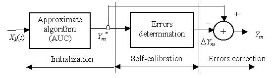
Fig. 1 self-correction algorithm of digital signal processing
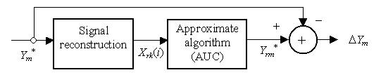
Fig. 2 Self-calibration of the algorithm under correction
To determine the calculation errors of the AUC, the original output parameters Y
m* are assigned as reference parameters for the self-calibration
(Fig.2). Using the reference parameters Ym* reconstruction
data Xrk(i) (k=1,2,..., K; i=0,1,..., N-1) are generated with
a corresponding model. Reference output parameters Yrm*
(m=1,2,..., M) are then estimated by the same AUC with the use of the reconstruction data X
rk(i). The errors of the parameters calculated by the AUC can be determined by
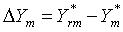
if the reconstruction data Xrk(i) can accurately be calculated
with the corresponding model. After the self-calibration errors correction is made by
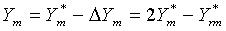
The calculation errors of the AUC can thus be self-corrected without any error analysis and
external reference.
Remark 1: The self-correction algorithm mentioned above bases on an accurately realizable
signal reconstruction without considering any signal noise. This condition limits the application
areas of the self-correction algorithm. For instance, this algorithm can be applied to a discrete
Fourier transform for processing spectral limited signals but not for spectral unlimited
signals, because a spectral unlimited signal cannot accurately be reconstructed with the inverse
Fourier transform due to the spectral leakage of higher frequency components.
Remark 2: The calculation errors of an approximate algorithm depends on the input signals
Xk(i). The reconstruction data Xrk(i)
are not the same of the input signals Xk(i), because the reference
parameter Ym* deviate from the true parameters. Therefore the
errors determined by the self-calibration are not the true errors caused by the approximate algorithm (AUC).
This is why a recursive/iterative self-correction algorithm has been proposed.
For processing signals interfered with noise, however, only the first few self-corrections are useful
for the accuracy improvement. The further iterative self-corrections are not necessary for processing
practical signals. In most cases up to 3 self-corrections are enough for the errors correction of an
approximate algorithm. As example Fig. 3 shows an algorithm that uses two self-corrections.
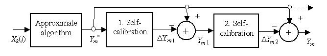
Fig.3 Scheme of an iterative self-correction algorithm
In this case the reference parameters Ym,1 for the second self-calibration
are more accurate to the true parameters than the reference parameters Yrm*
for the first self-calibration, so that the errors DYm,2
are more accurate to the true errors caused by the AUC in the initialization. The final output
parameters can be calculated by
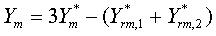
where Y*rm,1 and Y*rm,2
are the reference output parameters in the first and second self-calibrations, respectively.
Generally, the final output parameters of an iterative self-correction algorithm are written by
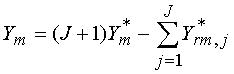
with J as the number of iterative self-corrections and Y*rm,j
as the reference output parameters in the j-th self-calibration.
Remark 3: The residual errors of the self-calibration algorithm depends on the original
parameter errors caused by the approximate algorithm. A larger residual error is caused by a larger original error.
All original errors of calculated parameters must be less than 70 %, otherwise errors convergence of
the self-calibration algorithm cannot be guaranteed. Therefore, it is useful to reduce the original
errors by using other methods in advance if the original errors are larger than the limit value.
These algorithms are applied to the discrete Fourier-Series/Transformation
(DFT) of periodic signals sampled asychronously and to
parameter estimation of damped oscillation signals.
|