Parameter determination of damped oscillation signals plays an important role in the technical
diagnosis of analog circuits and systems, and for the measurement and analysis of elektrical and
mechanical quantities.
A typical damped sinusoid oscillation signal can usually be written by
 (1) (1)
with A and j as beginning amplitude and phase,
b as damping factor, and xn(t) as noise.
The signal frequency f of the damped oscillation signal can firstly be estimated using the sampling
data via more than 2 signal periods. The parameters b, A and
j can then be determined by the following algorithm.
For parameter estimation, the oscillation signal is sampled via 2 periods. Each period contains
N samples. The sampling data are two-dimensionally numbered, i.e., x(i,j), i=0, 1, 2,..., N-1 and
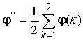
j=1, 2. The amplitudes A(k) and phases j(k), k=1,2, of each period are
calculated by a discrete Fourier transform. The value of the beginning phase j
* is resulted from the mean value:
 (2)
(2)
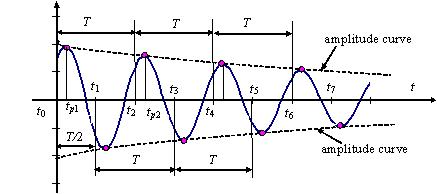 Fig. 1 Estimation of b* and A*
using the sampling data of the first two periods
Fig. 1 Estimation of b* and A*
using the sampling data of the first two periods
From Fig. 1 the damping factor b*
can be derived as: 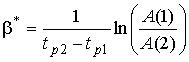 (3)
(3)
where tp1 and tp2 denote the time at the maximum of the sampled signal in
the first and second period, respectively.
The beginning amplitude A* is then determined by
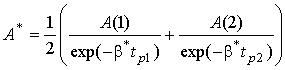 (4) (4)
For practical uses the parameter estimation algorithm mentioned above is not satisfying with
respect to its accuracy. The errors are caused by noise and the DFT due to signal damping and
asynchronous sampling. The noise influence on the parameter estimation can be reduced by an
averaging with the use of sampling data via more than 2 signal periods. The systematic errors
should be reduced by the self-correction algorithm (Fig. 2).
After a self-correction the parameters b, A, and
j are determined according to the self-correction:
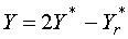 (Y=b, A, and j)
(5)
(Y=b, A, and j)
(5)
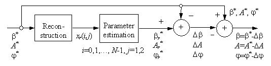 Fig. 2 Self-correction algorithm for compensating systematic errors of parameter
estimation
The final output parameters of an iterative self-correction algorithm are written by
Fig. 2 Self-correction algorithm for compensating systematic errors of parameter
estimation
The final output parameters of an iterative self-correction algorithm are written by
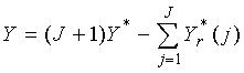 (Y=b, A, and j) (6)
with J as the number of iterative self-corrections and Y*r
(j) as reference output parameters in the j-th self-correction.
Different simulations are made by using the damped oscillation signal (1). The signal is sampled
asynchronously. Fig. 3 shows the simulation results calculated by the parameter estimation
algorithm without self-correction in the case of xn(t)=0. Calculation errors are caused
by the original algorithm and the asynchronous sampling. They increase with the asynchronous factor
a and decrease with the number of samples N per signal period.
The errors mentioned above can be compensated by the self-correction algorithm. Fig. 4 shows the
reduction errors of the parameters after the second iterative self-correction using (6) with J=2.
The relative errors are limited within ±0.02% for determining all three parameters both using
synchronous and asynchronous sampling data if noise is not considered.
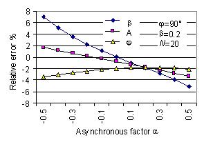
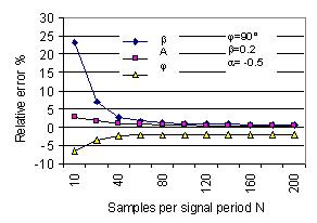
Fig. 3 Parameter estimation errors of damped signal (1) calculated by algorithm
without self-correction
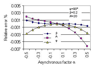
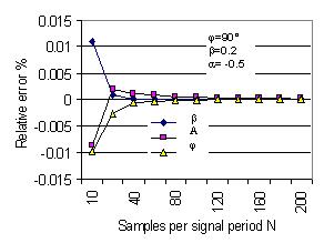
Fig. 4 Parameter estimation errors of damped signal (1) calculated by algorithm
with the self-correction
|