|
Fourier analysis is one of the most important signal processing methods in the measurement technolgy. Using the
Fourier analysis, the spectra of measuring signals can be determined, which play an important role
for the signal transfer, analysis, and filtering in measuring systems. Precise Fourier analysis is
widely used for the measurements of electrical, optic and mechanical quantities e.g. impedance,
transfer function, oscillations etc.
A discrete spectral limited periodic or periodically extended signal x(k) can be expressed by
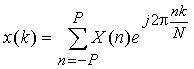 (1)
(1)
with
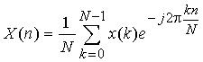 (2)
(2)
The samples x(k) (k=0, 1, 2, ..., N-1) at the discrete time k are expressed as products of
original signal samples and a rectangular time window of a length Tm
, where N denotes the number of samples contained within the time window.
X(n) (n= -P, ... , -2, -1, 0, 1, 2,..., P) are the corresponding frequency components with P as
the highest order of the harmonics. Equation (2) is known as the Discrete Fourier Transform (DFT)
and (1) the Inverse Discrete Fourier Transform (IDFT).
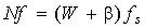
According to the sampling theorem the number of sampling points N must be more than the double of
the highest order P of the harmonics, i.e., N>2P. In this case the frequency components of a spectral
limited signal can accurately be calculated by the DFT if the signal is sampled synchronously
and the condition Wfs=Nf is fulfilled, where W is the number of
complete signal periods contained within the time window Tm.
The relation between the sampling and signal frequencies can generally be written by
 |b|<0.5 (3)
In this case the signal frequencies of the harmonics cannot accurately be determined by using
the time window Tm,
so that some frequency components cannot be found in the spectrum. The spectral-leakage occurs.
For W=1, i.e., the time window contains one signal period, a sampling condition is derived from (3),
and it can be written by
 |a|<0.5 (4)
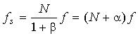
with N as the number of samples per signal period, and a as asynchronous factor.
For a=0 one obtains the synchronous sampling condition f
s=Nf. This condition is indispensable for the DFT because it is necessary to
fulfill the orthogonal condition of the DFT. The DFT cannot exactly be derived if the orthogonal
condition is failed.
In the case a>0 and a<0 the calculation
errors are caused by the DFT, even if the signal is spectral limited. These errors are caused by
asynchronous sampling and can also be considered as the spectral-leakage errors.
The errors mentioned above can be effectively reduced not only by interpolation in time domain,
but also by interpolation in frequency domain. The DFT algorithm with pre-processing by an
interpolation algorithm is known as Interpolated DFT (IP-DFT). In the data-synchronization
approach the asynchronous sampling data are synchronously re-sampled by an interpolation.
The re-sampled data are then processed by the DFT.
The interpolation errors, however, are not negligible for signal processing in measurement,
especially, in the case of a lower number of samples per signal period.
The calculation errors of the DFT can be self-corrected better by the
self-correction algorithm.
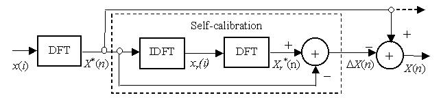
Fig. 1 Scheme of a self-corrected DFT algorithm
The self-correction DFT algorithm (SC-DFT) is shown in Fig. 1. The DFT is an approximate
algorithm under correction. The IDFT is used for the signal reconstruction.
For spectral limited signals the reconstruction data xr(i)
can accurately be calculated by the IDFT (1). The application condition is
fulfilled in this case. The final output frequency components can be written by
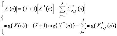 (5) (5)
(n= -P, ... , -2, -1, 0, 1, 2,..., P) where X*(n) is the
original frequency components calculated by the DFT using the input data x(i)
at the initialization, and X*r,j(n) denotes the j-th
reference output components determined by the DFT using the reconstructed data
xr,j(i) during the self-calibration. The self-calibration and
self-correction are separately implemented with the magnitude and phase components.
This can improve the speed of error reduction of an iterative self-correction algorithm.
As example Fig. 2 and 3 show results of computer simulations. The amplitude and phase errors of
a sinusoid signal calculated by the self-correction DFT are given in comparison
with those of the fundamental DFT and the Interpolated DFT. The signal is asynchronously sampled
in a time window of one signal period (W=1). The errors of the DFT
algorithms increase with the asynchronous factor a, and decrease inversely with the samples number
N. The calculation errors of the SC-DFT and IP-DFT are obviously less
than those of the fundamental DFT. The errors of the SC-DFT(1) using one self-correction are less
than those of the IP-DFT if N<15 for the amplitude and N<60 for the phase.
After two iterative self-corrections the errors of the SC-DFT(2) are less than those of the IP-DFT
for N<500.
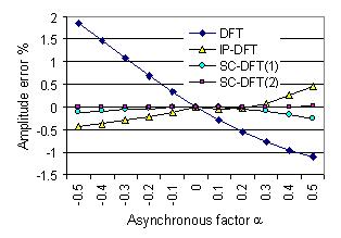
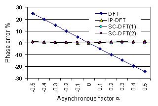
Fig. 2 Errors as function of the asynchronous factor a
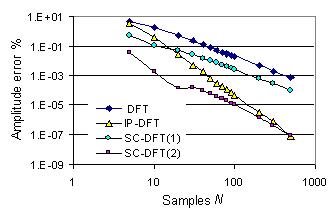
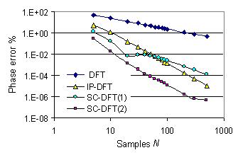
Fig. 3 Errors as function of the sampling point in one signal
|